R language standard distribution

In random collections of data from independent sources, the distribution of data is usually observed to be normal. T his means that when we draw a graph of the count of variable values on the horizontal axis and values on the vertical axis, we get a bell curve. T he center of the curve represents the average of the dataset. I n the figure, 50% of the values are on the left side of the average and the other 50% are on the right side of the chart. T his is statistically referred to as a normal distribution.

The R language has four built-in functions to produce a normal distribution. T hey are described below.

dnorm(x, mean, sd)
pnorm(x, mean, sd)
qnorm(p, mean, sd)
rnorm(n, mean, sd)

The following is a description of the parameters used in the above features -

• x is the vector of the number.

• p is the vector of probability.

• n is the number of observations (sample size).

• mean is the average of the sample data. I ts default value is zero.

• sd is a standard deviation. I ts default value is 1.

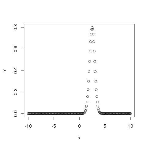
dnorm（）

The function gives the height of the probability distribution of a given mean and standard deviation at each point.

# Create a sequence of numbers between -10 and 10 incrementing by 0.1.
x <- seq(-10, 10, by = .1)

# Choose the mean as 2.5 and standard deviation as 0.5.
y <- dnorm(x, mean = 2.5, sd = 0.5)

# Give the chart file a name.
png(file = "dnorm.png")

plot(x,y)

# Save the file.
dev.off()

When we execute the code above, it produces the following results -

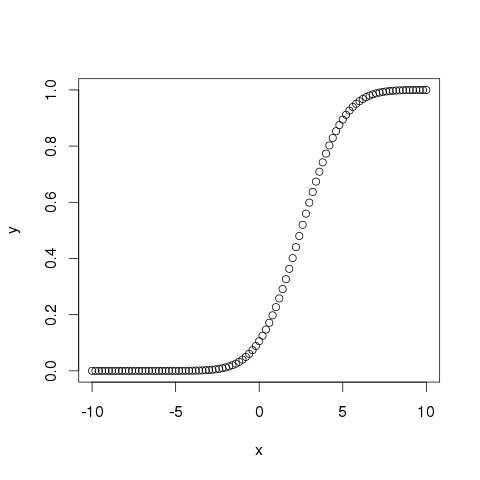
pnorm（）

The function gives the probability that the normal distribution random number is less than the value of a given number. I t is also known as a "cumulative distribution function."

# Create a sequence of numbers between -10 and 10 incrementing by 0.2.
x <- seq(-10,10,by = .2)
 
# Choose the mean as 2.5 and standard deviation as 2. 
y <- pnorm(x, mean = 2.5, sd = 2)

# Give the chart file a name.
png(file = "pnorm.png")

# Plot the graph.
plot(x,y)

# Save the file.
dev.off()

When we execute the code above, it produces the following results -

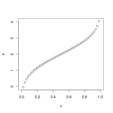
qnorm（）

The function takes the probability value and gives the number that the cumulative value matches the probability value.

# Create a sequence of probability values incrementing by 0.02.
x <- seq(0, 1, by = 0.02)

# Choose the mean as 2 and standard deviation as 3.
y <- qnorm(x, mean = 2, sd = 1)

# Give the chart file a name.
png(file = "qnorm.png")

# Plot the graph.
plot(x,y)

# Save the file.
dev.off()

When we execute the code above, it produces the following results -

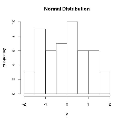
RNORM（）

This function is used to generate random numbers that are normally distributed. I t takes the sample size as input and generates many random numbers. L et's draw a histogram to show the distribution of the resulting numbers.

# Create a sample of 50 numbers which are normally distributed.
y <- rnorm(50)

# Give the chart file a name.
png(file = "rnorm.png")

# Plot the histogram for this sample.
hist(y, main = "Normal DIstribution")

# Save the file.
dev.off()

When we execute the code above, it produces the following results -