R language time series analysis

Time series is to arrange the uniform statistical values according to the order in which the time occurs, and the main purpose of time series analysis is to predict the future based on the available data.

A stable time series often consists of two parts, that is: a regular time series and noise. Therefore, in the following methods, the main purpose is to filter the noise values, so that our time series more analytical significance.

Grammar

The basic syntax of the ts() function in time series analysis is -

timeseries.object.name <-  ts(data, start, end, frequency)

The following is a description of the parameters used -

• data is a vector or matrix of values that are included in a time series.

• Start specifies the start time of the first observation in a time series.

• End specifies the end time of the last observation in the time series.

• Frequency specifies the number of observations per unit of time.

All parameters are optional except the parameter "data".

Pre-processing of time series:

1. Smoothness test:

   After we get a time series, we must first judge its stability, only the stability time series of non-white noise can have the significance of analysis and predict the value of future data.

   The so-called stability, refers to the statistical value fluctuates up and down a constant and the range of fluctuations is bounded. I f there is a clear trend or periodicity, then it is unstable. There are three ways to generally judge:

   • Draw a trend chart of the time series and see the trend judgment
   • Draw self-correlation and partial correlation diagrams, self-correlation and partial correlation diagrams for smooth time series, either tailed or cut.
   • Check for unit roots in the sequence, or non-smooth time series if unit roots exist.

   In the R language, DF detection is a method of detecting stability, and if the resulting P-value is less than the critical value, the sequence is considered stable.

2. White noise test

   White noise sequence, also known as pure random sequence, there is no correlation between the values of the sequence, sequence in disorderly random fluctuations, can terminate the analysis of the sequence, because the white noise sequence is not able to extract any valuable information.

3. The parameter characteristics of a smooth time series

   The average and variance are constants and have time-independent self-co-concierconciation variances.

Time series modeling steps:

• Get the time series dataset being analyzed.
• For data mapping, observe its smoothness. I f a non-smooth time series is first performed by d-order differential operation and then turned into a smooth time series, the d here is d in the ARIMA (p, d, q) model, and if it is a smooth sequence, the ARMA (p, q) model is used. S o what distinguishes the ARIMA (p,d,q) model from ARMA (p,q) is that the feature polynism of the self-regression part of the former contains d unit roots.
• The resulting smooth time series obtained its self-correlation coefficient ACF and partial correlation coefficient PACF respectively, and obtained the best class p and order q by analyzing the self-correlation graph and partial correlation graph. T he ARIMA model is obtained from d, q, and p above.
• Model diagnostics. D iagnostic analysis was carried out to confirm that the resulting model did match the observed data characteristics. If not, go back to step (3).

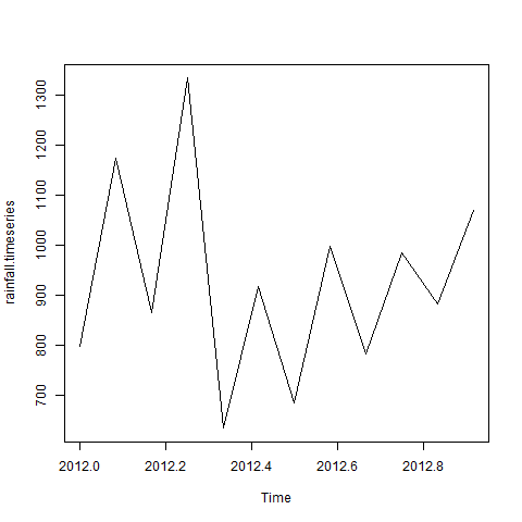
Cases

Consider the details of the annual rainfall in a place starting in January 2012. We create an R time series object for 12 months and draw it.

# Get the data points in form of a R vector.
rainfall <- c(799,1174.8,865.1,1334.6,635.4,918.5,685.5,998.6,784.2,985,882.8,1071)

# Convert it to a time series object.
rainfall.timeseries <- ts(rainfall,start = c(2012,1),frequency = 12)

# Print the timeseries data.
print(rainfall.timeseries)

# Give the chart file a name.
png(file = "rainfall.png")

# Plot a graph of the time series.
plot(rainfall.timeseries)

# Save the file.
dev.off()

When we execute the code above, it produces the following results and charts -

Jan    Feb    Mar    Apr    May     Jun    Jul    Aug    Sep
2012  799.0  1174.8  865.1  1334.6  635.4  918.5  685.5  998.6  784.2
        Oct    Nov    Dec
2012  985.0  882.8 1071.0

Time series chart -

Different time intervals

The frequency parameter value in the ts() function determines the time interval at which the data point is measured. A value of 12 indicates a time series of 12 months. O ther values and their meanings are as follows -

• Frequency : 12 specifies the data points for each month of the year.

• Frequency : 4 data points per quarter of each year.

• Frequency : 10 minutes of data points per hour of 6 hours.

• The frequency is 24 x 6 fixed every 10 minutes of the day.

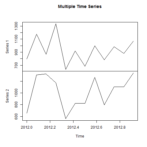
Multi-time series

We can plot multiple time series in a single chart by combining two series into a matrix.

# Get the data points in form of a R vector.
rainfall1 <- c(799,1174.8,865.1,1334.6,635.4,918.5,685.5,998.6,784.2,985,882.8,1071)
rainfall2 <- 
           c(655,1306.9,1323.4,1172.2,562.2,824,822.4,1265.5,799.6,1105.6,1106.7,1337.8)

# Convert them to a matrix.
combined.rainfall <-  matrix(c(rainfall1,rainfall2),nrow = 12)

# Convert it to a time series object.
rainfall.timeseries <- ts(combined.rainfall,start = c(2012,1),frequency = 12)

# Print the timeseries data.
print(rainfall.timeseries)

# Give the chart file a name.
png(file = "rainfall_combined.png")

# Plot a graph of the time series.
plot(rainfall.timeseries, main = "Multiple Time Series")

# Save the file.
dev.off()

When we execute the code above, it produces the following results and charts -

           Series 1  Series 2
Jan 2012    799.0    655.0
Feb 2012   1174.8   1306.9
Mar 2012    865.1   1323.4
Apr 2012   1334.6   1172.2
May 2012    635.4    562.2
Jun 2012    918.5    824.0
Jul 2012    685.5    822.4
Aug 2012    998.6   1265.5
Sep 2012    784.2    799.6
Oct 2012    985.0   1105.6
Nov 2012    882.8   1106.7
Dec 2012   1071.0   1337.8

Multi-time series chart -