R Language Survival Analysis

Survival Analysis handles predicting when a particular event will occur. I t is also known as failure time analysis or analysis of death time. F or example, predict how many days a person with cancer will survive or predict how long the mechanical system will fail.

The R language pack named survival is used for survival analysis. T his package contains the function Surface(), which uses the input data as an R-language formula and creates a survival object in the selected variable for analysis. T hen we use the function survfit() to create an analysis diagram.

Install the package

install.packages("survival")

Grammar

The basic syntax for creating survival analysis in the R language is -

Surv(time,event)
survfit(formula)

The following is a description of the parameters used -

• Time is the tracking time until the event occurs.

• Event indicates the state in which the expected event occurred.

• Formula is the relationship between predictors.

Cases

We'll consider a dataset called "pbc" that exists in the survival package installed above. I t describes survival data points for people affected by hepatic primary bile cirrhosis (PBC). O f the many columns that exist in the data set, we focus on the fields "time" and "status". T ime represents the number of days between the registration of a patient receiving a liver transplant or a patient's death and the earlier event.

# Load the library.
library("survival")

# Print first few rows.
print(head(pbc))

When we execute the code above, it produces the following results and charts -

  id time status trt      age sex ascites hepato spiders edema bili chol
1  1  400      2   1 58.76523   f       1      1       1   1.0 14.5  261
2  2 4500      0   1 56.44627   f       0      1       1   0.0  1.1  302
3  3 1012      2   1 70.07255   m       0      0       0   0.5  1.4  176
4  4 1925      2   1 54.74059   f       0      1       1   0.5  1.8  244
5  5 1504      1   2 38.10541   f       0      1       1   0.0  3.4  279
6  6 2503      2   2 66.25873   f       0      1       0   0.0  0.8  248
  albumin copper alk.phos    ast trig platelet protime stage
1    2.60    156   1718.0 137.95  172      190    12.2     4
2    4.14     54   7394.8 113.52   88      221    10.6     3
3    3.48    210    516.0  96.10   55      151    12.0     4
4    2.54     64   6121.8  60.63   92      183    10.3     4
5    3.53    143    671.0 113.15   72      136    10.9     3
6    3.98     50    944.0  93.00   63       NA    11.0     3

From the above data, we are considering the time and status of the analysis.

Apply the Surv() and survfit() functions

Now let's continue to apply the Surv() function to the dataset above and create a trend chart that will show.

# Load the library.
library("survival")

# Create the survival object. 
survfit(Surv(pbc$time,pbc$status == 2)~1)

# Give the chart file a name.
png(file = "survival.png")

# Plot the graph. 
plot(survfit(Surv(pbc$time,pbc$status == 2)~1))

# Save the file.
dev.off()

When we execute the code above, it produces the following results and charts -

Call: survfit(formula = Surv(pbc$time, pbc$status == 2) ~ 1)

      n  events  median 0.95LCL 0.95UCL 
    418     161    3395    3090    3853 

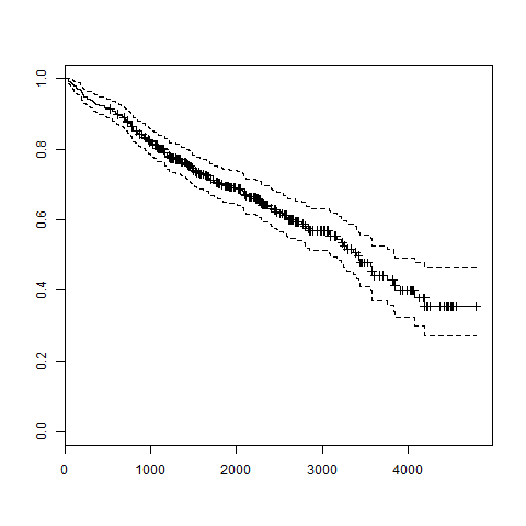
The trends in the figure above help us predict the probability of survival at the end of a particular number of days.